This report analyzes a full year of gold mill performance using a realistic ore-processing dataset. The goal was to evaluate recovery efficiency, tailings losses, feed grade behavior, and overall process stability using Power BI. Through interactive dashboards, trend charts, KPIs, and correlation analysis, the report highlights how operational variables such as ore hardness, grind size, and feed grade impact recovery and gold loss. This project demonstrates my ability to model complex industrial data, build meaningful KPIs, and extract insights that support data-driven decision-making in mining operations.
Objective:
The objective of this project is to analyze and optimize the metallurgical performance of a gold-processing operation by developing a realistic 12-month ore-processing dataset and transforming it into a comprehensive Power BI dashboard. The project aims to evaluate gold recovery efficiency, identify factors contributing to metallurgical losses, and highlight relationships between key process variables such as ore hardness, grind size, feed grade, tailings grade, and mill performance.
Through the integration of Python-based data modeling and Power BI visualization, the goal is to create actionable insights that support decision-making, improve gold recovery, reduce tailings losses, and enhance overall plant stability. This project demonstrates the ability to build mining-industry datasets, design KPIs, and apply analytical methods to solve complex process and operational challenges.
Data Collection & Preparation
Dataset Overview:
In this project, we used Python to:
- Generate a 12-month ore-processing dataset
- Simulate realistic metallurgy behavior (recovery vs tailings)
- Model ore hardness, grind size, mill power, feed grade
- Add statistical noise to reflect real mining variability
- Ensure correlations (e.g., hardness → grind → tailings → recovery)
Dataset contains 1,000 daily ore-processing records including feed grade, hardness (BWi), tons processed, mill power, grind size (P80), gold recovery %, and tailings grade. Data reflects real mine behavior with accurate metallurgical relationships used for recovery and loss analysis.
Columns: Date ,Feed_Grade_gpt, Ore_Hardness_BWi_kWh_t, Tons_Processed, Mill_Power_kW, Pulp_Density_pct, Grind_Size_P80_microns,Tailings_Grade_gpt, Gold_Recovery_pct
import pandas as pd
import numpy as np
from datetime import datetime, timedelta

# Parameters
n = 1000
start_date = datetime(2024, 1, 1)

# Generate dates (daily or every 9 hours)
dates = [start_date + timedelta(hours=9*i) for i in range(n)]

# Feed grade (g/t) – realistic gold ore
feed_grade = np.random.uniform(2.0, 6.5, n)

# Ore hardness (Bond Work Index)
hardness = np.random.normal(14, 2.5, n).clip(8, 22)

# Tons processed – decreases with harder ore
tons_processed = (
    4200 - (hardness - 12) * 80 + np.random.normal(0, 150, n)
).clip(2500, 5000)

# True metallurgical recovery (89–96%)
true_recovery = np.random.uniform(0.89, 0.96, n)

# Tailings grade derived from feed grade + recovery relationship
tailings_grade = feed_grade * (1 - true_recovery)

# Gold recovery percent
gold_recovery_pct = true_recovery * 100

# Mill power – higher hardness = higher mill power draw
mill_power = (
    3800 + (hardness - 12) * 150 + np.random.normal(0, 120, n)
).clip(2500, 6000)

# Pulp density (% solids)
pulp_density = np.random.uniform(30, 45, n)

# Grind size (P80 microns)
grind_size = np.random.normal(75 + (hardness - 14) * 2, 8, n).clip(40, 150)

# Build DataFrame
df = pd.DataFrame({
    "Date": dates,
    "Feed_Grade_gpt": np.round(feed_grade, 3),
    "Ore_Hardness_BWi_kWh_t": np.round(hardness, 2),
    "Tons_Processed": np.round(tons_processed),
    "Mill_Power_kW": np.round(mill_power),
    "Pulp_Density_pct": np.round(pulp_density, 1),
    "Grind_Size_P80_microns": np.round(grind_size, 1),
    "Tailings_Grade_gpt": np.round(tailings_grade, 3),
    "Gold_Recovery_pct": np.round(gold_recovery_pct, 2)
})

# Save to Excel
df.to_excel("OreProcessing_REALISTIC_1000rows.xlsx", index=False)

df.head()
Dataset Sample:

KPIs Calculations:
Metallurgical & Ore Processing KPIs – Summary Table
| KPI Name | Description | DAX Measure |
|---|---|---|
| Total_Tons_Processed | Total ore tonnage processed over the selected period. | Total_Tons_Processed = SUM('Data'[Tons_Processed]) |
| Avg_Gold_Recovery | Average gold recovery % over the selected period. | Avg_Gold_Recovery = AVERAGE('Data'[Gold_Recovery_pct]) |
| Avg_Tailings_Grade | Average gold grade in tailings (g/t). Indicates long-term metal loss. | Avg_Tailings_Grade = AVERAGE('Data'[Tailings_Grade_gpt]) |
| Gold_Lost_g | Total grams of gold lost to tailings (metallurgical loss). | Gold_Lost_g = SUMX('Data', 'Data'[Tons_Processed] * 'Data'[Tailings_Grade_gpt]) |
| Gold_Recovered_g | Total grams of gold recovered by the plant. | Gold_Recovered_g = SUMX('Data', 'Data'[Tons_Processed] * ('Data'[Feed_Grade_gpt] - 'Data'[Tailings_Grade_gpt])) |
| kW_per_Ton | Energy intensity of grinding: kW drawn per ton processed. Lower = more efficient. | kW_per_Ton = DIVIDE(SUM('Data'[Mill_Power_kW]), SUM('Data'[Tons_Processed])) |
| Tons_per_kW | Tons processed per kW used. Higher = better energy efficiency. | Tons_per_kW = DIVIDE(SUM('Data'[Tons_Processed]), SUM('Data'[Mill_Power_kW])) |
| Avg_Hardness | Average ore hardness (Bond Work Index, kWh/t). | Avg_Hardness = AVERAGE('Data'[Ore_Hardness_BWi_kWh_t]) |
| Tailings_Ratio_% | % of gold remaining in tailings relative to feed grade (loss ratio). | Tailings_Ratio_% = AVERAGEX('Data', 100 * ('Data'[Tailings_Grade_gpt] / 'Data'[Feed_Grade_gpt])) |
| Gold_Recovery_30Day | Rolling 30-day average gold recovery. Smooths daily noise and shows trend. | Gold_Recovery_30Day = AVERAGEX(DATESINPERIOD('Data'[Date], MAX('Data'[Date]), -30, DAY), 'Data'[Gold_Recovery_pct]) |
| Recovery_StdDev | Standard deviation of gold recovery. Measures recovery stability. | Recovery_StdDev = STDEV.P('Data'[Gold_Recovery_pct]) |
Analysis & Visualizations
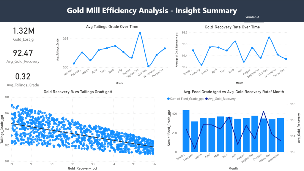
Key Insights:
Gold Recovery Stability (92.2% – 92.7%)
Gold Recovery remained consistently stable across the 12-month period, averaging approximately 92.5%.
Minor fluctuations occurred month-to-month, which is normal for an underground gold operation where ore hardness, grind size, and feed variability naturally change.
- Highest recovery: October–November
- Lowest recovery: February and July
- Trend: Strong operational stability overall
This indicates good control of the grinding, leaching, and recovery processes.
Tailings Grade Trend
- Tailings Grade fluctuated between 0.30–0.36 g/t, with peaks in March, July, and October, indicating periods of suboptimal liberation or leaching.
Recovery Over Time
- Recovery peaks occurred in June, August, and November, suggesting periods of better ore characteristics or improved operating conditions.
- February and July dips indicate possible harder ore or less efficient grinding/leach conditions.
Feed Grade Relationship
- Higher Feed Grades generally showed slightly higher recovery performance, but the relationship is modest—indicating good operational control regardless of ore grade variation.
- Slight dips early in the year
- Improvement toward mid-year
- Stable grade during final months
Recovery increased slightly during higher-grade months, consistent with improved gold mass pull and leach kinetics.
Tailings Grade vs Recovery (Strong Inverse Correlation)
scatter plot clearly shows a strong negative correlation between:
- The downward trend confirms strong metallurgical behavior: when recovery increases, tailings grade decreases.
- Consistent pattern across 1,000+ samples shows stable process control with predictable gold loss trends.
Dashboard Summary:
- The mill operated with high metallurgical stability and minimal volatility.
- Recovery is mainly driven by tailings performance, not feed grade or hardness alone.
- Seasonal dips may indicate:
- harder ore feed in winter months
- reduced grinding efficiency
- lower temperatures affecting leach kinetics
- October shows peak performance—possibly due to:
- softer ore
- optimized grind size
- steady feed characteristics
- improved reagent or leach management
Conclusion
This project demonstrates a complete end-to-end analysis of a gold-processing operation using a realistic 12-month metallurgical dataset. By combining Python for data modeling and Power BI for visualization, the analysis successfully highlights key relationships between recovery performance, tailings losses, ore hardness, grind size, feed grade, and energy consumption.
The resulting dashboard provides clear visibility into operational trends, identifies the drivers behind recovery fluctuations, and quantifies the impact of tailings on metallurgical losses. Through KPI modeling, correlation analysis, and rolling performance metrics, the project delivers actionable insights that can support decision-making, improve recovery consistency, and reduce gold losses in real mining operations.






 CYBERWARD
Leave a comment